Day 3 - Bacterial Pangenomics
The exercises of day one and day two were centered around relatively small data / genomes. Now, day three moves on to - bacteria!
The objectives were two-fold: we were provided with whole genome and single gene sequences and were supposed to create a graph of a single gene and build a graph-based pangenome. Then we should have figured out ways to learn if a gene is present or absent in a strain, and identify a set of genes present in all strains (the core genome) versus genes that are missing in some strains (accessory genes).
In the course we were working with E. coli data that Mikko had prepared for us. I am going to work with Pseudomonas aeruginosa instead, since the objectives (except maybe for the single gene graph) are my work goals as well, so I can use this to start working on my own data.
- Getting started
- Pseudomonas aeruginosa references
- “Pangenome” graph based on five reference genomes
- Open questions
Getting started
I have a protocol from the course as inspiration, in addition to the actual course materials, where we extracted sequences of gyrA from all provided E. coli strains to create a graph, and then moved on to create a whole genome graph using 10 random E. coli strains. The latter we used to map the gyrA fasta sequence to see where it was located in the graph, and we also mapped provided short reads and all gene sequences of a not included strain to the “pangenome”.
Pseudomonas aeruginosa references
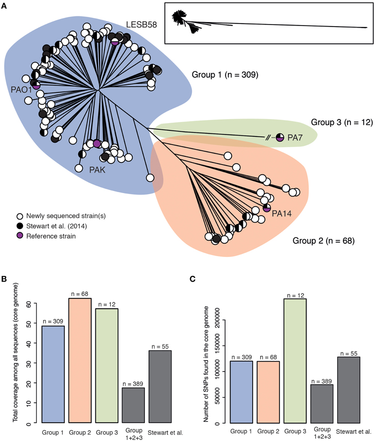
I’m going to do something similar here. I’ll start with a few reference sequences from pseudmonas.com; there are 208 strains with complete genomes included in the database right now, while NCBI lists 209 complete genomes. We usually use P. aeruginosa PA14 as reference, or PAO1 (which is the recommended standard), and in phylogenetic trees we use strains from the popular five on pseudomonas.com (PAO1, PA14, LESB58, PA7). In general, it seems that most sets of P. aeruginosa strains can be divided into “PA14-like” and “PAO1-like” strains and a small group of outliers related to PA7. The PAO1 group usually includes most other reference strains as well (e.g. here, here, or here).
“Pangenome” graph based on five reference genomes
To start, I will create a genome graph based on the top five P. aeruginosa reference strains, and depending on how long that takes I can then think about using all 208 strains instead. Since P. aeruginosa has a well conserved genome, it might not even be necessary to use so many whole genomes - augmenting the starting graph with missing sequences and variations could also be a good strategy.
mkdir day3
cd day3/
mkdir pics
mkdir references
cd references/
wget http://pseudomonas.com/downloads/pseudomonas/pgd_r_19_1/Pseudomonas_aeruginosa_PAO1_107/Pseudomonas_aeruginosa_PAO1_107.fna.gz
wget http://pseudomonas.com/downloads/pseudomonas/pgd_r_19_1/Pseudomonas_aeruginosa_UCBPP-PA14_109/Pseudomonas_aeruginosa_UCBPP-PA14_109.fna.gz
wget http://pseudomonas.com/downloads/pseudomonas/pgd_r_19_1/Pseudomonas_aeruginosa_LESB58_125/Pseudomonas_aeruginosa_LESB58_125.fna.gz
wget http://pseudomonas.com/downloads/pseudomonas/pgd_r_19_1/Pseudomonas_aeruginosa_PA7_119/Pseudomonas_aeruginosa_PA7_119.fna.gz
wget http://pseudomonas.com/downloads/pseudomonas/pgd_r_19_1/Pseudomonas_aeruginosa_PAK_6441/Pseudomonas_aeruginosa_PAK_6441.fna.gz
gunzip *.gz
Case in point: the group that created PPanGGOLiN, a different pangenome graph approach, analysed 3958 P. aeruginosa genomes from GenBank and found a quite large “soft core” genome (as shown in the publication).
Graph creation with minimap2 and seqwish
As I’ve already seen in day two that using vg msga can be quite slow when creating a graph based on multiple genomes, I’m going to use the minimap2+seqwish approach again. Since the genomes are circular in Pseudomonas anyway, there shouldn’t be any confusion about that this time.
First, I have to combine the five fasta sequence files into one multi-fasta file:
for i in $(ls *fna)
do
  cat $i >> FivePsae.fasta
done
Now I can run minimap2 to do the alignment and then use seqwish to create a graph from that:
minimap2 -X -c -x asm20 FivePsae.fasta FivePsae.fasta | gzip > FivePsae.paf.gz
seqwish -s FivePsae.fasta -p FivePsae.paf.gz -b FivePsae.work -g FivePsae.gfa | pv -l
I’m still using the -x asm20 for lack of a better idea. Very useful is also the option to pipe in gzip to create a compressed output and save some space.
[M::mm_idx_gen::1.495*1.00] collected minimizers
[M::mm_idx_gen::1.695*1.23] sorted minimizers
[M::main::1.695*1.23] loaded/built the index for 5 target sequence(s)
[M::mm_mapopt_update::1.796*1.21] mid_occ = 100
[M::mm_idx_stat] kmer size: 19; skip: 10; is_hpc: 0; #seq: 5
[M::mm_idx_stat::1.860*1.21] distinct minimizers: 2341228 (48.14% are singletons); average occurrences: 2.504; average spacing: 5.506
[M::worker_pipeline::19.029*2.24] mapped 5 sequences
[M::main] Version: 2.17-r954-dirty
[M::main] CMD: minimap2 -X -c -x asm20 FivePsae.fasta FivePsae.fasta
[M::main] Real time: 19.072 sec; CPU: 42.664 sec; Peak RSS: 0.868 GB
Creating the alignment was again very fast (19 seconds), so I believe that adding at least a few more genomes wouldn’t be a problem. Since seqwish doesn’t include output with run time, I’ve included | pv -l in my call to be able to accurately stop the time.
0 0:01:09 [ 0 /s] [<=> ]
This is a pretty handy tool, and shows that seqwish is also really fast (one minute) for the five reference genomes.
Graph visualisation
Of course I now want to take a look at my P. aeruginosa mini-pangenome! I’ll start with odgi, but I’m probably going to use vg viz as well.
odgi build -g FivePsae.gfa -o - | odgi sort -i - -o FivePsae.og
odgi viz -i FivePsae.og -o ../pics/FivePsae.png -x 2000 -R
Again, odgi viz gives out some additional information about the paths in the graph:
path 0 refseq|NC_011770|chromosome 0.65 0.152778 0.197222 249 58 75
path 1 refseq|NC_009656.1|chromosome 0.254032 0.254032 0.491935 97 97 188
path 2 refseq|NZ_CP020659.1|chromosome 0.474088 0.0690979 0.456814 181 26 175
path 3 refseq|NC_002516.2|chromosome 0.460952 0.48 0.0590476 176 184 23
path 4 refseq|NC_008463.1|chromosome 0.430809 0.0443864 0.524804 165 17 20
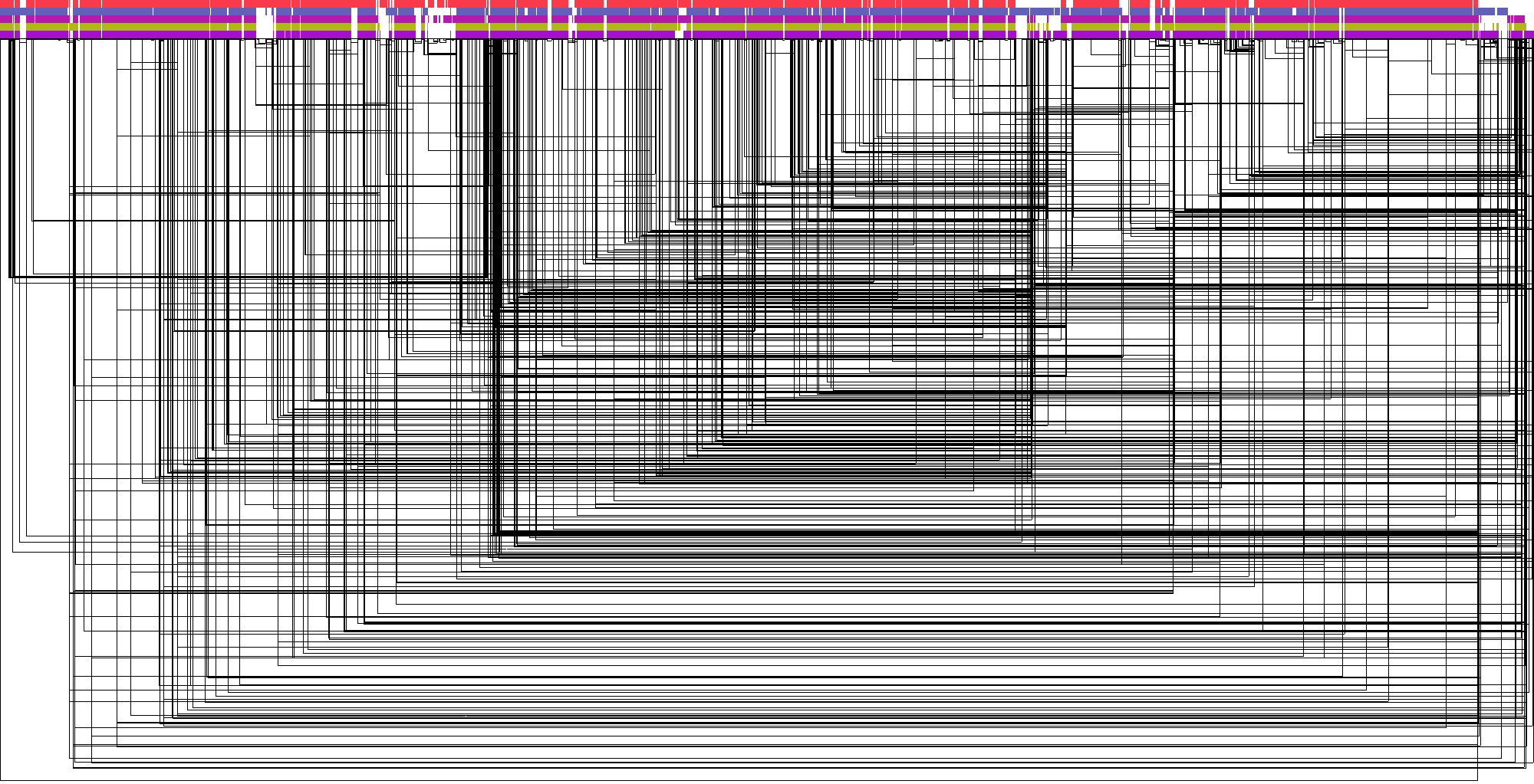
pangenome graph based on five references
There are a lot of edges in this graph, and while odgi viz creates a nice overview of this, I think vg viz is better if you want to see some details (like which genome is which).
vg view -F FivePsae.gfa -v > FivePsae.vg
vg index -x FivePsae.xg FivePsae.vg
vg viz -x FivePsae.xg -o ../pics/FivePsae.svg
These steps take a little time, but now I have an SVG file that I can load into Inkscape to check out… and it’s empty. I can’t see any graph inside, just the border box that’s usually around the image. I wonder where the graph got lost - let’s find it!
File sizes of my different graph formats:
| format | size |
|---|---|
| GFA | 97M |
| OG | 92M |
| VG | 28M |
| XG | 136M |
Hmm, the vg graph is a lot smaller than the other two, but the index is big and at least for day two, the graph created with seqwish and then converted to vg looks similar (size wise). The conversion had worked there, too, as I was able to map reads to the converted graph.
What does the vg file look like, then? Let’s ask jq:
vg view FivePsae.vg -j | jq ".path"
Great, paths are there just fine. Maybe the whole graph is too big for vg viz? I’ll try looking at just a few nodes instead.
Since jq listed a bunch of nodes to the console for me, I can just choose a number from there:
vg find -n 668831 -x FivePsae.xg -c 10 | vg view -dp - | dot -Tpdf -o ../pics/FivePsae_668831.pdf
That is also working perfectly: DOT version of node 668831 and surroundings (PDF)
So now I know that the graph and the index are fine, and it’s vg viz that… can’t cope with the amount of data?
vg find -n 668831 -x FivePsae.xg -c 10 | vg view -v - > FivePsae_668831.vg
vg index -x FivePsae_668831.xg FivePsae_668831.vg
vg viz -x FivePsae_668831.xg -o ../pics/FivePsae_668831.svg
Apparently yes, since this worked fine as well:
vg viz version of node 668831 and surroundings
There is yet another visualisation tool that I have not yet tested, but we’re very interested in: IVG, which creates sequence tube maps. Sadly, this online tool can only take uploads of up to 5 MB, and apparently it can’t deal with graphs that only contain a few extracted nodes, either:
terminate called after throwing an instance of 'std::runtime_error' what(): Attempted to get handle for node 101 not present in graph ERROR: Signal 6 occurred. VG has crashed. Run 'vg bugs --new' to report a bug. Stack trace path: /tmp/vg_crash_aQ6V67/stacktrace.txt
Apparently my only way to look at the graph is using odgi viz (or just looking at parts and not the whole thing). Since the additional output of odgi viz lists the path identities, at least I believe I know which genome is which:
| path | colour | RefSeq | name |
|---|---|---|---|
| 0 | red | NC_011770 | LESB58 |
| 1 | blue | NC_009656.1 | PA7 |
| 2 | pink | NZ_CP020659.1 | PAK |
| 3 | green | NC_002516.2 | PAO1 |
| 4 | purple | NC_008463.1 | PA14 |
Scrolling through the graph, there are multiple regions visible which are specific for a single genome, mostly for LESB58, but also for PA7 and PAK. I’m a little surprised that LESB58 seems to be so different from the others, since it usually clusters with PAO1 and PAK, while PA7 is always shown as a - very different - outlier. Of course, the coloured paths are basically just the multiple sequence alignment and the edges show the real genome composition in the end - only they are very hard to interpret in this format.
Annotating the graph
Before I move on to mapping samples to the graph, I would like to be able to identify genes and other features of the reference genomes in the graph. Similar to my analysis of HIV I could then also look at “variation” in the genes, based on the number of nodes per gene. My problem here is that I have five annotated references that make up the graph, and many of the annotated genes will be the same (remember, big soft core genome). Since vg gives each gene its own path, I assume it would be a bit too much to augment the graph with all five complete annotations. Instead, I want to try and create one annotation for all five references.
First, I’ll download the annotations for all five in GFF3 format, since vg needs GFF (or BED, but that’s not listed on pseudomonas.com):
mkdir annotations
cd annotations
wget http://pseudomonas.com/downloads/pseudomonas/pgd_r_19_1/Pseudomonas_aeruginosa_PAO1_107/Pseudomonas_aeruginosa_PAO1_107.gff.gz
wget http://pseudomonas.com/downloads/pseudomonas/pgd_r_19_1/Pseudomonas_aeruginosa_UCBPP-PA14_109/Pseudomonas_aeruginosa_UCBPP-PA14_109.gff.gz
wget http://pseudomonas.com/downloads/pseudomonas/pgd_r_19_1/Pseudomonas_aeruginosa_LESB58_125/Pseudomonas_aeruginosa_LESB58_125.gff.gz
wget http://pseudomonas.com/downloads/pseudomonas/pgd_r_19_1/Pseudomonas_aeruginosa_PA7_119/Pseudomonas_aeruginosa_PA7_119.gff.gz
wget http://pseudomonas.com/downloads/pseudomonas/pgd_r_19_1/Pseudomonas_aeruginosa_PAK_6441/Pseudomonas_aeruginosa_PAK_6441.gff.gz
gunzip *.gz
Since I don’t want to do a homology search or anything, I’ll keep it “simple”: I’ll look for gene names and if they are the same in multiple files, I’ll keep only one of them. I will also sort through the gene/CDS duplicates and probably only keep the gene entries if start and stop are equivalent to a CDS entry.
There will be another problem, though: the GFF files I downloaded start every entry with “chromosome” as seqid instead of a valid RefSeq or other identifier for the genomes. I don’t think that will work with vg annotate, but I’ll check first:
vg annotate -x FivePsae.xg -f annotations/Pseudomonas_aeruginosa_PAO1_107.gff > FivePsaePAO1.gam
warning: path "chromosome" not found in index, skipping
No, it’s not working. So here is what I have/want to accomplish using a Python script:
- exchange “chromosome” with an actual path/reference name
- maybe change the path names from “
refseq|NC_011770|chromosome” to just “NC_011770” using jq first?
- maybe change the path names from “
- remove duplicate gene/CDS entries
- filter genes in different references so every gene is only annotated once (or at least most genes are)
Preparing the annotation
I decided to keep the path names as they are to save some time. The Python script I wrote (using Python 3) is called CleanMergeGff.py and resides in the same directory as the annotation files. The script reads a file listing GFF files to clean and combine, ignores features that are not needed, removes duplicate gene/CDS entries and only keeps one gene annotation for all references (based on gene name).
python3 CleanMergeGff.py annot_list.tab
wc -l PseudomonasAnnotation.gff
25187 PseudomonasAnnotation.gff
Each single annotation file contains between 11,000 and 13,000 entries, while the combined annotation file contains only 25,000 hopefully unique entries. Now let’s add those to the variant graph.
cd ../
vg annotate -x FivePsae.xg -f annotations/PseudomonasAnnotation.gff > FivePsaeAnnot.gam
vg augment FivePsae.vg -i FivePsaeAnnot.gam > FivePsaeAnnot.vg
vg index -x FivePsaeAnnot.xg FivePsaeAnnot.vg
The annotation is really fast, while augmentation and indexing take some time. Again, we can’t possibly visualise the whole graph with all the paths, so I have to select a region I want to visualise. This can be done using vg paths, which - I believe - can select paths by name from a variant graph:
vg paths -x FivePsaeAnnot.xg -X -Q "gyrA" > FivePsaeAnnotgyrA.gam
Again (similar to vg annotate in day two, vg paths does not create a vg output file even when given the -V option - it turns out as gam anyway, so I’m using -X (to create a gam file) just to be consistent. The output file does not contain any paths, though - interesting…
vg paths -x FivePsaeAnnot.xg -L
This command is supposed to list all paths in the file. The output is this:
refseq|NC_002516.2|chromosome
refseq|NC_008463.1|chromosome
refseq|NC_009656.1|chromosome
refseq|NC_011770|chromosome
refseq|NZ_CP020659.1|chromosome
Since vg annotate did not complain about the annotation format or seqid (first column in the gff), I assumed that everything worked this time, but the annotation does not seem to be there.
What is inside FivePsaeAnnot.gam, then?
vg view -a FivePsaeAnnot.gam | jq '.path' > FivePsaeAnnotPaths.json
I tried to have a look at the gam file after conversion to json using tidyjson, but I get an error in return:
Error: parse error: trailing garbage
          "393756"       }     }   ] } {   "mapping": [     {       "e
                     (right here) ------^
Something seems to have gone wrong in this file somewhere, even though there was no previous error message.
Does something similar happen when I just try to annotate one of the references?
In order to figure that out, I have to adjust an annotation file to have the right seqid (fitting one of the paths in the variant graph), which I’m just going to do manually with the PAO1 annotation.
vg annotate -x FivePsae.xg -f annotations/Pseudomonas_aeruginosa_PAO1_107_corrected.gff > FivePsaePAO1Annot.gam
vg augment FivePsae.vg -i FivePsaePAO1Annot.gam > FivePsaePAO1Annot.vg
vg index -x FivePsaePAO1Annot.xg FivePsaePAO1Annot.vg
vg paths -x FivePsaePAO1Annot.xg -L
Pseudomonas aeruginosa PAO1 refseq|NC_002516.2|chromosome, complete genome.
refseq|NC_002516.2|chromosome
refseq|NC_008463.1|chromosome
refseq|NC_009656.1|chromosome
refseq|NC_011770|chromosome
refseq|NZ_CP020659.1|chromosome
OK, so now I have one single path from the annotation, that is new. I did exactly the same thing for the HIV data, and when I use vg paths -L on these data, I get a list of two paths per gene, just as I saw in the visualisation. Why is this not happening here? It’s not like I updated vg or anything, so the software didn’t change.
For some reason vg annotate took only the first line from my PAO1 gff file and annotated that into the graph, right? I think I’d like to have a look at that…
vg paths -x FivePsaePAO1Annot.xg -X -Q "Pseudomonas aeruginosa PAO1 refseq|NC_002516.2|chromosome, complete genome." > FivePsaePAO1Annotpath.gam
Since this file is now supposed to only contain parts of the graph that contain the path I chose, I should be able to get any random node ID from it (or the json version of it) and visualise that.
vg view -a FivePsaePAO1Annotpath.gam | jq '.path'
vg find -n 489302 -x FivePsaePAO1Annot.xg -c 10 | vg view -v - > FivePsaePAO1Annot_489302.vg
vg index -x FivePsaePAO1Annot_489302.xg FivePsaePAO1Annot_489302.vg
vg viz -x FivePsaePAO1Annot_489302.xg -o ../pics/FivePsaePAO1Annot_489302.svg
graph path 'Pseudomonas aeruginosa PAO1 refseq|NC_002516.2|chromosome, complete genome.' invalid: edge from 489292 start to 489312 end does not exist
graph path 'Pseudomonas aeruginosa PAO1 refseq|NC_002516.2|chromosome, complete genome.' invalid: edge from 489292 start to 489312 end does not exist
[vg view] warning: graph is invalid!
Despite a warning from the vg find command, this code works:
vg viz version of node 489302 and surroundings
Right, so in general I know what I have to do. Now the question remains why it doesn’t work as expected, and I have an idea - there is one interesting difference between the gff file I downloaded for HIV and the one for PAO1 (or any of the other reference strains): every line in the bacterial annotation ends with a semicolon (semicolons separate the entries in the attributes string), while the HIV annotation does not have a semicolon at the end of a line. Maybe that is taken as a sign that the annotated entry is not finished yet?
I’m going to remove the trailing semicolons from the already corrected PAO1 annotation and try again:
vg annotate -x FivePsae.xg -f annotations/Pseudomonas_aeruginosa_PAO1_107_corrected.gff > FivePsaePAO1Annot.gam
vg augment FivePsae.vg -i FivePsaePAO1Annot.gam > FivePsaePAO1Annot.vg
vg paths -v FivePsaePAO1Annot.vg -L
refseq|NC_002516.2|chromosome
refseq|NC_008463.1|chromosome
refseq|NC_009656.1|chromosome
refseq|NC_011770|chromosome
refseq|NZ_CP020659.1|chromosome
Interesting! We’re down again to the five original paths, with nothing new added. This must somehow be related to the format of my files, but I struggle to see it. Both the HIV annotation and my file have LF line breaks according to Notepad++, both are tab separated files with the same number of columns.
In the attributes column there is one more difference I only noticed now after checking out the GFF specifications: their tags usually start with a capital letter, which is only partly true in the HIV annotation (but true for all features that were annotated in the graph) and only partly true in PAO1, where the official (?) “name” tag does not start with a capital “N” as expected, except for in the first entry… Could it be that stupid?
vg annotate -x FivePsae.xg -f annotations/Pseudomonas_aeruginosa_PAO1_107_corrected.gff > FivePsaePAO1Annot.gam
vg augment FivePsae.vg -i FivePsaePAO1Annot.gam > FivePsaePAO1Annot.vg
vg paths -v FivePsaePAO1Annot.vg -L
And suddenly I have a loooong list of paths in my annotated graph! I need emojis in this protocol…
I still don’t understand why the version without trailing semicolons didn’t even get the first feature annotated, but that’s a question for another day and for now I just hope it’s not a relevant one.
For now, I’ve adjusted my Python script to correct the formatting of my gff files:
python3 CleanMergeGff.py annot_list.tab
cd ../
vg annotate -x FivePsae.xg -f annotations/PseudomonasAnnotation.gff > FivePsaeAnnot.gam
vg augment FivePsae.vg -i FivePsaeAnnot.gam > FivePsaeAnnot.vg
vg paths -v FivePsaeAnnot.vg -L
Working with an annotated graph
It worked!
Time to look at some genes. The gene list I just got ended with “zwf”, “zwf1”, and “zwf2”, I’m curious enough about that to start with those.
vg index -x FivePsaeAnnot.xg FivePsaeAnnot.vg
vg paths -x FivePsaeAnnot.xg -X -Q "zwf" > FivePsaeAnnotZwf.gam
vg view -a FivePsaeAnnotZwf.gam | jq '.path' > FivePsaeAnnotZwf_path.jq
Extracting the paths for those genes (-Q in vg paths sets the “name prefix”, so I can find all three genes) is really quick, and there don’t seem to be many nodes involved.
Luckily, we extracted all nodes for certain paths on day 4 of the course and I have the jq command to do it (I don’t know how long it would have taken me to figure it out by myself).
vg view -a FivePsaeAnnotZwf.gam | jq '{name: .name, nodes: ([.path.mapping[].position.node_id | tostring] | join(","))}'
zwf1 has by far the most nodes, and I think I would have to load this into R, or at least sort it somewhere to get an overview, because the node IDs jump around a lot (e.g. “1109132,1019278,688979,1019279,688981,1019280,688983”). I’ll just have a look at a random location:
vg find -n 1019278 -x FivePsaeAnnot.xg -c 10 | vg view -v - > FivePsaeAnnot_1019278.vg
vg index -x FivePsaeAnnot_1019278.xg FivePsaeAnnot_1019278.vg
vg viz -x FivePsaeAnnot_1019278.xg -o ../pics/FivePsaeAnnot_1019278.svg
vg view -dp FivePsaeAnnot_1019278.vg | dot -Tpdf -o ../pics/FivePsaeAnnot_1019278.pdf
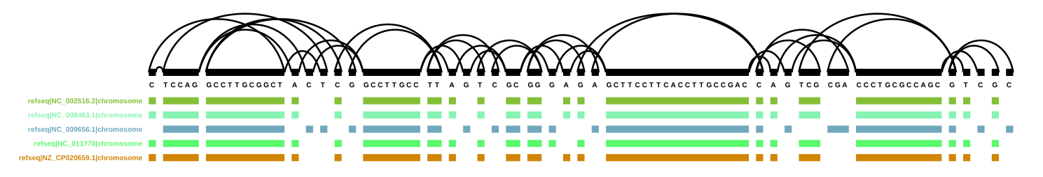
vg viz version of node 1019278 and surroundings
DOT version of node 1019278 and surroundings (PDF)
Cool, it worked! I already wish I could select which tag will be used as path name, though… Gene names are fine (although it would be cool to also have the information in which genome this gene is now officially annotated), but the protein/product names are a bit annoying.
Beside that, we can easily see (in the SVG/PNG version) that this is not the best way to look at specific genes inside the graph - the nodes are sorted by node ID, and the list of IDs already showed that the gene itself is not represented in a linear set of nodes.
My chosen example, zwf1 (the purple path at the bottom), is a gene from PA7 (NC_009656.1, the light blue middle of the reference paths), but does - even in this small example - not touch all nodes that the PA7 genome touches.
The DOT version looks quite different from the SVG version. Here, the node IDs are displayed, which helps in navigating the graph. Together with other genes (cdhA, phzC2, pys2, and QueF), the path for zwf1 only starts in the middle of the depicted region. This is what I would actually have expected, since the gene starts at node 1109132 and then touches node 1019278, which is the node I selected (and therefore the numeric middle of the displayed region). I wonder how vg viz decides what to display and in which order…
So, being aware of the different visualisation methods and their quirks is important if you want to visually inspect your graph (or parts of it).
With regards to the actual content of these visualisations - I think I would really have to see the whole gene. Why? Because of all the other genes starting(?) at the same node - none of them are listed as orthologs for zwf1 on pseudomonas.com. I have to see the whole gene.
Luckily, vg find could actually be able to do that, using the -N (node list file) option instead of -n (node ID). Since I don’t want to create another GAM file for only zwf1, I’m going to write all three paths to the file and manually remove the two I’m not interested in right now.
vg view -a FivePsaeAnnotZwf.gam | jq '{name: .name, nodes: ([.path.mapping[].position.node_id | tostring] | join(","))}' > zwf_nodes.txt
vg find -N zwf1_nodes.txt -x FivePsaeAnnot.xg -c 10 | vg view -v - > FivePsaeAnnot_zwf1.vg
vg index -x FivePsaeAnnot_zwf1.xg FivePsaeAnnot_zwf1.vg
vg viz -x FivePsaeAnnot_zwf1.xg -o ../pics/FivePsaeAnnot_zwf1.svg
vg view -dp FivePsaeAnnot_zwf1.vg | dot -Tpdf -o ../pics/FivePsaeAnnot_zwf1.pdf
graph path 'GDP-mannose 4,6-dehydratase (pseudogene)' invalid: edge from 1142390 start to 1120667 end does not exist
[vg view] warning: graph is invalid!
Again I got a warning when using vg find - or, more correctly, vg view, as I got the same error when converting to DOT format - to create a sub-graph. I assume that not all nodes for this specific path were included in my list. Creating the DOT format also takes a lot of time and cannot be recommended for this (sub-)graph size any more. Creation of an SVG is quick, but opening it in Inkscape is not.
A quick glance using Internet Explorer (I am forced to use this to remotely connect to our server in Braunschweig) shows that there are a lot of paths and a lot of edges between the nodes which presumably make rendering difficult for many programs.
Since it will be hard to analyse this visually/manually, I’ll try to look at this programmatically. My nodespergene.R script from day 2 is a good start for that, using the FivePsaeAnnot_zwf1.vg file that I also used for the visualisation of the sub-graph.
vg view FivePsaeAnnot_zwf1.vg -j > FivePsaeAnnot_zwf1.json
jq '.path' FivePsaeAnnot_zwf1.json > FivePsaeAnnot_zwf1_paths.json
graph path 'GDP-mannose 4,6-dehydratase (pseudogene)' invalid: edge from 1142390 start to 1120667 end does not exist
[vg view] warning: graph is invalid!
Is it bad that I’m getting used to ignoring these kinds of errors?
I wrote I quick R script to have a look at the paths in this sub-graph - or more specifically at zwf1, cdhA, phzC2 and pys2.
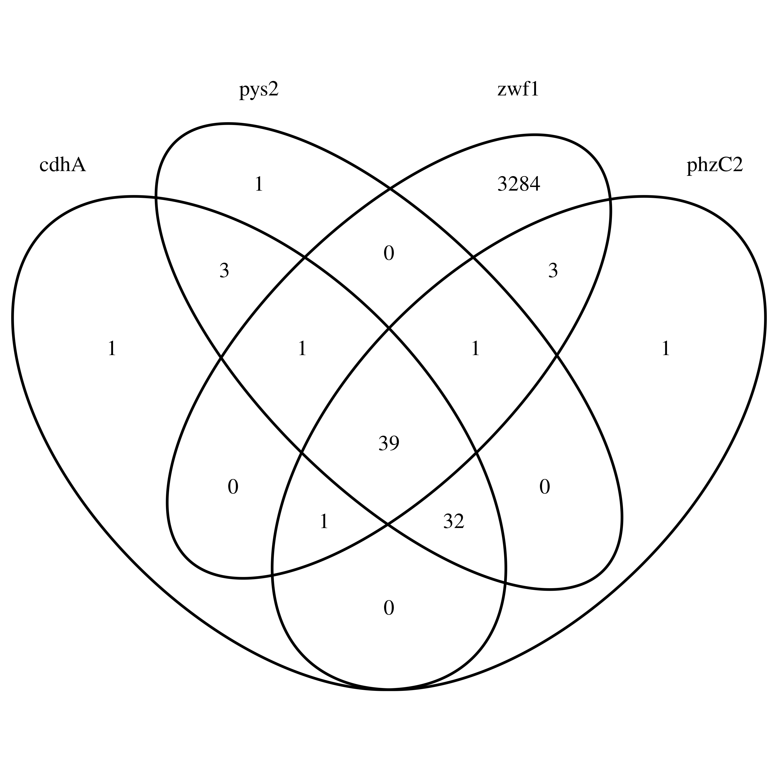
Venn diagram of zwf1, cdhA, phzC2 and pys2
Each gene has at least one node that distinguishes it from the others. Additionally, zwf1 has a lot more nodes than the other three genes.
Looking at all paths included in this sub-graph, zwf1 has by far the most nodes (3329, compared to 647 of the gene with the next most nodes), except for the reference genomes, which all contain more than 4000 nodes here. This is interesting, since I set vg find to use the nodes touched by zwf1, but obviously more nodes are included…?
Caveats
As I’ve already seen when I extracted zwf1 from the whole graph, the nodes that make up this gene’s paths are not in a numerical order. Since the node IDs are so far apart (1109132,1019278,688979,…), I assume that the nodes are created per genome/path, so zwf1 touches nodes that came with different references. The problem I see here is with my approach to merge the annotations - for example, I have now one annotated version of oprD, but I know there are phylogenetic differences in the different strain versions. So how well would I be able to find “everything” that is oprD in such an approach?
To test this, and to generally get a “data-driven” feeling for this problem, I’m going to create a mini-annotation with all versions of oprD (manually) and annotate the graph with that.
Note: oprD is not a core gene, and PAK has a number of “OprD family” annotated genes, but none with the gene name oprD, so I’ll leave that strain out for now.
vg annotate -x FivePsae.xg -f annotations/oprD_annotation.gff > FivePsaeoprD.gam
vg augment FivePsae.vg -i FivePsaeoprD.gam > FivePsaeoprD.vg
vg index -x FivePsaeoprD.xg FivePsaeoprD.vg
vg paths -x FivePsaeoprD.xg -X -Q "oprD" > FivePsaeoprD_path.gam
vg view -a FivePsaeoprD_path.gam | jq '{name: .name, nodes: ([.path.mapping[].position.node_id | tostring] | join(","))}' > oprD_nodes.txt
Great, I have the gam file with only the oprD path in it. Wait, with only one path? Well, yes, since the name is always the same, the information is… what? Merged into a single path? Or is the path always being replaced? Let’s check!
I replaced the “Name” in the annotation with the “Name”” and the “Alias” (the locus tag) separated by an underscore (so that I’m able to extract all the paths with “oprD” in them), so now I should be able to generate four paths.
vg annotate -x FivePsae.xg -f annotations/oprD_annotation2.gff > FivePsaeoprD2.gam
vg augment FivePsae.vg -i FivePsaeoprD2.gam > FivePsaeoprD2.vg
vg index -x FivePsaeoprD2.xg FivePsaeoprD2.vg
vg paths -x FivePsaeoprD2.xg -X -Q "oprD" > FivePsaeoprD2_path.gam
vg view -a FivePsaeoprD2_path.gam | jq '{name: .name, nodes: ([.path.mapping[].position.node_id | tostring] | join(","))}' > oprD2_nodes.txt
OK, now I can extract the paths and nodes for another visualisation.
vg view FivePsaeoprD.vg -j > FivePsaeoprD.json
jq '.path' FivePsaeoprD.json > FivePsaeoprD_paths.json
graph path 'oprD' invalid: edge from 1104943 end to 1104948 start does not exist
graph path 'oprD' invalid: edge from 1104943 end to 1104947 start does not exist
graph path 'oprD' invalid: edge from 1104941 end to 1104948 start does not exist
[vg view] warning: graph is invalid!
Ah, here we go again with the warnings. Will they come up with the second version as well? That would be a hint, indicating that maybe the path does get overwritten when the same name appears multiple times (when they don’t appear with properly separated paths).
vg view FivePsaeoprD2.vg -j > FivePsaeoprD2.json
jq '.path' FivePsaeoprD2.json > FivePsaeoprD2_paths.json
No error this time. What happens in the other version, then? The node IDs for all versions of oprD are saved somewhere, but not in the path information I extracted, so nodes are missing?
vg find -N oprD_nodes_clean.txt -x FivePsaeoprD.xg -c 10 | vg view -v - > FivePsaeoprD_nodes.vg
This results in a lot of errors. A few excerpts of all the different kinds are listed below:
[vg] warning: node ID 495199 appears multiple times. Skipping.
[vg] warning: node ID 495200 appears multiple times. Skipping.
[vg] warning: node ID 931098 appears multiple times. Skipping.
[vg] warning: edge 495199 end <-> 495200 start appears multiple times. Skipping.
[vg] warning: edge 931097 end <-> 495200 start appears multiple times. Skipping.
[vg] warning: edge 495200 end <-> 495201 start appears multiple times. Skipping.
[vg] warning: path oprD rank 39 appears multiple times. Skipping.
[vg] warning: path oprD rank 40 appears multiple times. Skipping.
[vg] warning: path oprD rank 42 appears multiple times. Skipping.
[vg] warning: path refseq|NC_002516.2|chromosome rank 13 appears multiple times. Skipping.
[vg] warning: path refseq|NC_002516.2|chromosome rank 14 appears multiple times. Skipping.
[vg] warning: path refseq|NC_002516.2|chromosome rank 15 appears multiple times. Skipping.
graph path 'oprD' invalid: edge from 1104943 end to 1104948 start does not exist
graph path 'oprD' invalid: edge from 1104943 end to 1104947 start does not exist
graph path 'oprD' invalid: edge from 1104941 end to 1104948 start does not exist
[vg view] warning: graph is invalid!
So the information is not overwritten in the xg index, but maybe in the json file? I’m only guessing here, though.
vg index -x FivePsaeoprD_nodes.xg FivePsaeoprD_nodes.vg
vg viz -x FivePsaeoprD_nodes.xg -o ../pics/FivePsaeoprD_nodes.svg
vg view -dp FivePsaeoprD_nodes.vg | dot -Tpdf -o ../pics/FivePsaeoprD_nodes.pdf
graph path 'oprD' invalid: edge from 1104943 end to 1104948 start does not exist
graph path 'oprD' invalid: edge from 1104943 end to 1104947 start does not exist
graph path 'oprD' invalid: edge from 1104941 end to 1104948 start does not exist
[vg view] warning: graph is invalid!
Warning: Could not load "/usr/bin/miniconda3/lib/graphviz/libgvplugin_pango.so.6" - It was found, so perhaps one of its dependents was not.  Try ldd.
Warning: Could not load "/usr/bin/miniconda3/lib/graphviz/libgvplugin_pango.so.6" - It was found, so perhaps one of its dependents was not.  Try ldd.
Format: "pdf" not recognized. Use one of: canon cmap cmapx cmapx_np dot dot_json eps fig gv imap imap_np ismap json json0 mp pdf pic plain plain-ext png pov ps ps2 svg svgz tk vdx vml vmlz xdot xdot1.2 xdot1.4 xdot_json
Again the invalid paths come up here, and apparently we now have problems with GraphViz so I can’t use the dot format. I’ll try to resolve this after creating the same sub-graph for all four paths of oprD.
vg find -N oprD2_nodes_unique.txt -x FivePsaeoprD2.xg -c 10 | vg view -v - > FivePsaeoprD2_nodes.vg
vg index -x FivePsaeoprD2_nodes.xg FivePsaeoprD2_nodes.vg
vg viz -x FivePsaeoprD2_nodes.xg -o ../pics/FivePsaeoprD2_nodes.svg
This ran without any error messages, so I now have the svg files for both versions of oprD (one path and four).
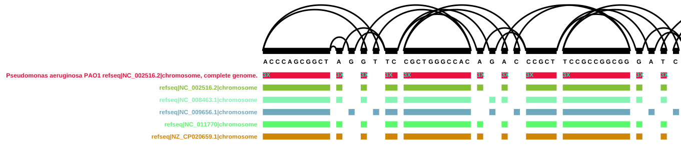
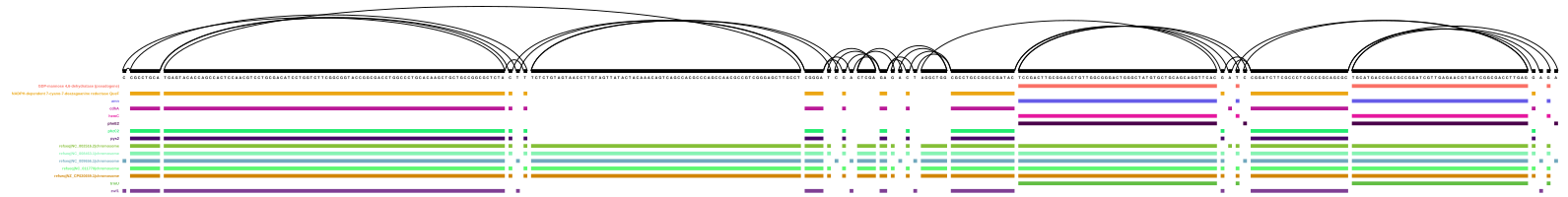
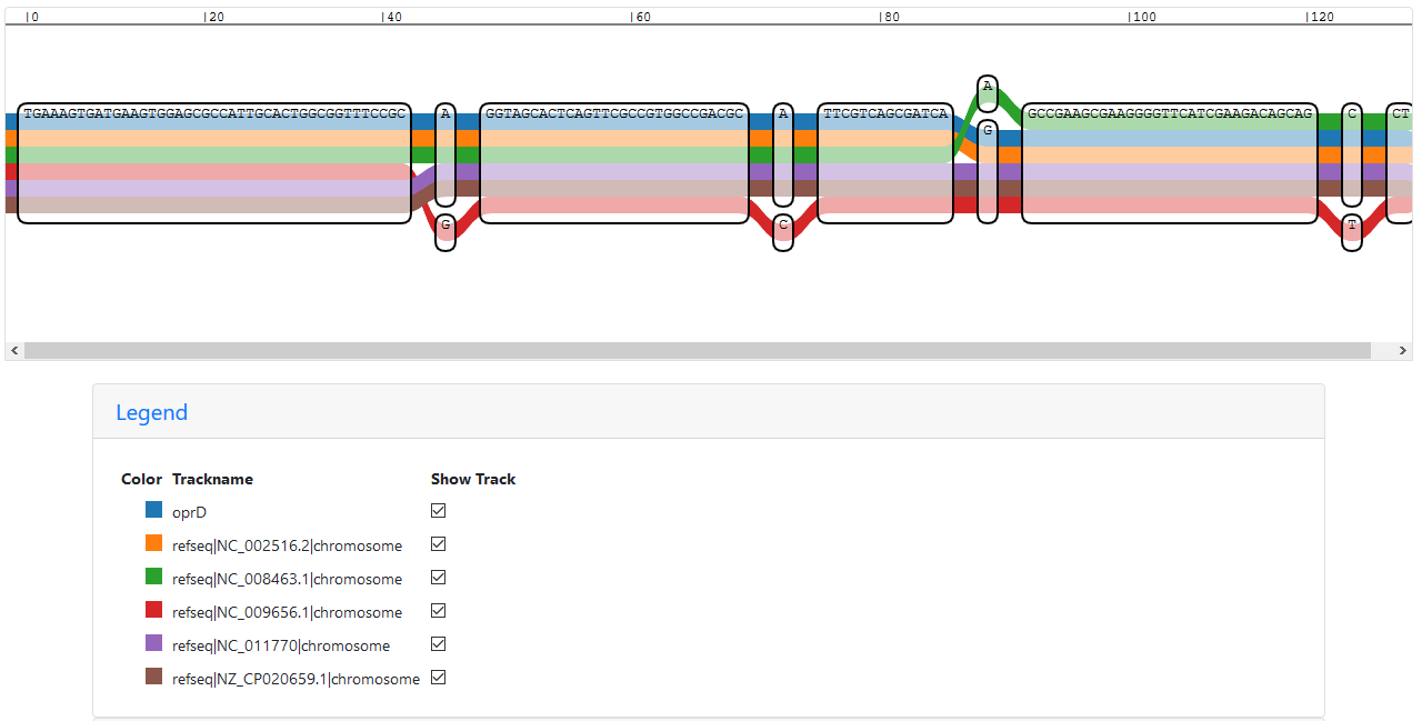
Start of the vg viz representation of a sub-graph with a merged oprD path
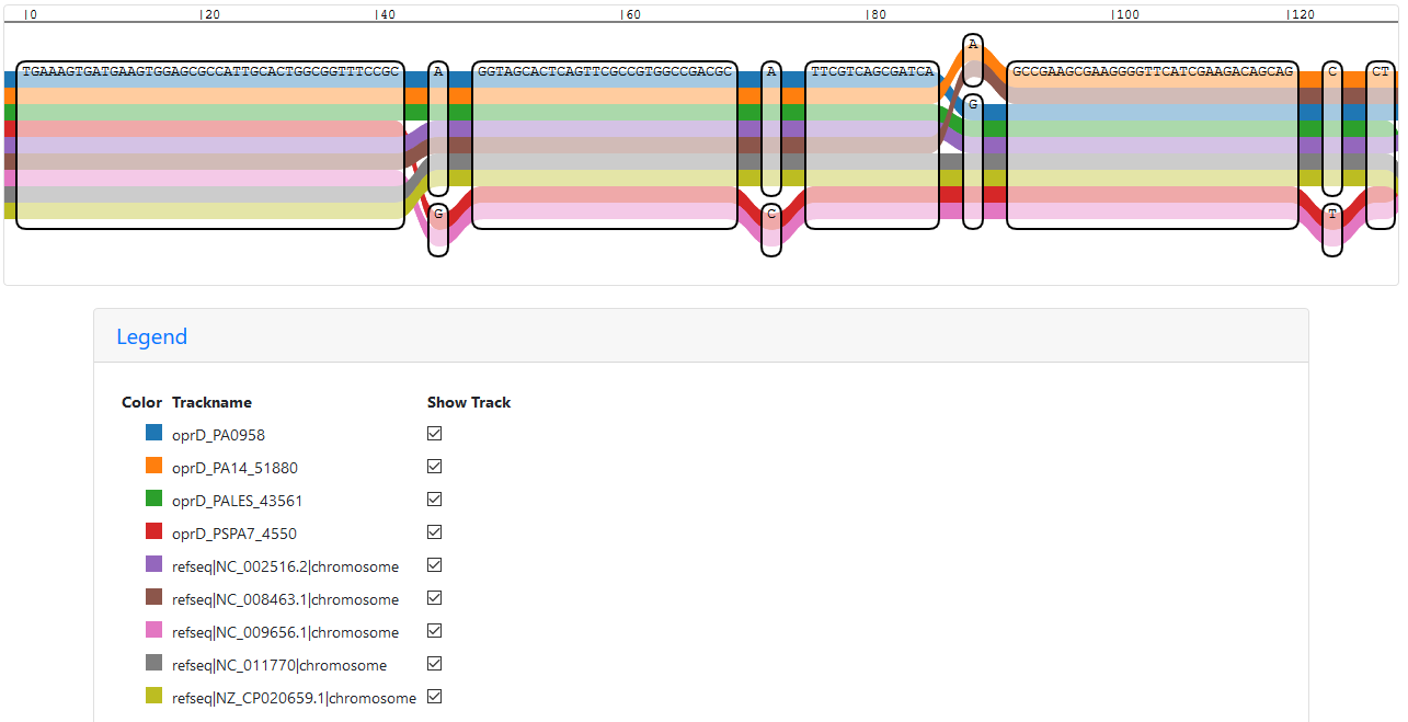
Start of the vg viz representation of a sub-graph with four oprD paths
This graph representation nicely shows that nodes are covered multiple times by the merged oprD path. It’s a bit difficult to directly compare it to the graph with the four oprD paths, since the order of the nodes is different, but I think it’s safe to presume that the number of repeats for a node correlates to the number of actual paths going through it in the second graph.
I also used the Sequence Tube Map online tool to visualise my sub-graphs in a different format. Here, the nodes are in the same order, but the number of repetition per node is not shown.
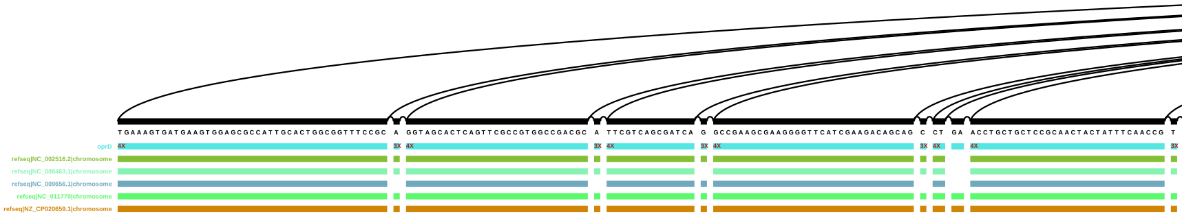
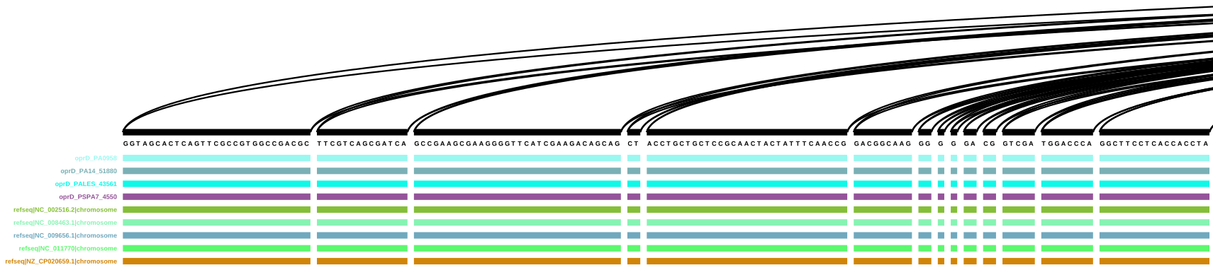
Start of the IVG representation of a sub-graph with a merged oprD path
Start of the IVG representation of a sub-graph with four oprD paths
When scrolling through the graph with only one oprD path, it’s interesting to see that the path is not following a single reference path, but instead seems to jump from one genome to the next. I assume that (at least in this tool?) part of the information does get overwritten, so if at one position the path should hit multiple nodes, only one is selected (but how?). In these cases, the vg viz representation is much clearer - if not all paths hit a node, the number of hits/repetitions for oprD goes down as well. Since the genomic position information is missing here, there is no conflict with two nodes being touched simultaneously.
Differences in visual representation aside, my main interest here was to see which nodes are touched by oprD and if a merging of reference annotations makes sense or not.
It doesn’t. If I want to know which “type” of oprD I have in my sample, I want to be able to evaluate all known paths the gene can take, so I need to know all nodes that were touched. This means two things:
- I cannot merge the reference annotations, so there will be a lot more paths than I hoped.
- I have to adjust the annotations again, to avoid duplicate gene names.
What’s the problem with duplicate gene names? They would basically lead to what I wanted in the beginning: one path instead of multiple. The merged path of oprD contains all nodes from the four separate paths, so I wouldn’t loose any information. On the other hand, I’d gain a lot of error messages for duplicates (which I could clean up, of course), and visualisation would be even more tricky. Mostly, though, I like to easily be able to see from which reference the path I’m hitting with an isolate originates (e.g. “is this the PA14 oprD or the PAO1 oprD?”).
Annotating everything
Well then, time to annotate everything and see how that works! I’ll write a CleanCombineGff.py script based on my previous annotation merging script for that.
Side note 1: A realisation I had while preparing the script for the new annotation is that there are actually a lot of times when the “Name” attribute in my GFF files is empty, which could in theory have led to empty path names and multiple paths being joined into one.
Side note 2: There were multiple problems with my annotation files, usually due to semicolons in the attributes where no semicolons should go, so I had to manually edit files in order for the script to run.
cd annotations/
python CleanCombineGff.py annot_list.tab
cd ..
vg annotate -x FivePsae.xg -f annotations/PseudomonasAnnotationAll.gff > FivePsaeAnnotAll.gam
Error parsing gtf/gff line 28618: refseq|NC_008463.1|chromosome P
Error parsing gtf/gff line 28717: refseq|NC_008463.1|chromosome P
Error parsing gtf/gff line 29480: refseq|NC_008463.1|chromosome P
There were a lot more of these error lines, so apparently I made a mistake in the annotation creation. I don’t know how this happened, but apparently I have a lot of lines that end at the “P” shown in the error message, instead of containing a whole annotation line. Huh, that is a strange outcome.
I probably should have used python3 instead of python when calling the script, as I got a new error from the script now (because I used “iteritems” instead of “items” at one point). This alone did not resolve the problem, though.
Which is no surprise, really, as the problem was in the last part of my code. I either have a string or a list item to write to my output file, and when I treat both as a list time (and index with “[0]”, as I did), I will only get the first letter from the string. I changed my list comprehension to get a string from there as well, to avoid this problem. This is one of a few parts of the script I’m not happy with, as it’s so specialised to these GFF files, but I can’t think of a generalisation right now.
cd annotations/
python3 CleanCombineGff.py annot_list.tab
cd ..
vg annotate -x FivePsae.xg -f annotations/PseudomonasAnnotationAll.gff > FivePsaeAnnotAll.gam
vg augment FivePsae.vg -i FivePsaeAnnotAll.gam > FivePsaeAnnotAll.vg
vg index -x FivePsaeAnnotAll.xg FivePsaeAnnotAll.vg
vg paths -v FivePsaeAnnot.vg -L | wc -l
vg paths -v FivePsaeAnnotAll.vg -L | wc -l
The file annotated with the reduced annotation contains 3497 paths, the new one with all features annotated contains 30578 paths. While this is a lot, the file sizes of the vg graphs are not so different, with 144M and 153M, respectively. At least this annotation should provide me with all information I need to analyse the features of my selected reference genomes and find them in our clinical isolates.
Can I also now use it to find “the real” oprD of the PAK genome in my graph?
vg paths -x FivePsaeAnnotAll.xg -X -Q "oprD" > FivePsaeAnnotAlloprD.gam
vg view -a FivePsaeAnnotAlloprD.gam | jq -r '([.path.mapping[].position.node_id | unique | tostring] | join("\n"))' > oprDAll_nodes.txt
vg find -N oprDAll_nodes.txt -x FivePsaeAnnotAll.xg -c 10 | vg view -v - > FivePsaeAnnotAlloprD_nodes.vg
vg index -x FivePsaeAnnotAlloprD_nodes.xg FivePsaeAnnotAlloprD_nodes.vg
vg viz -x FivePsaeAnnotAlloprD_nodes.xg -o ../pics/FivePsaeAnnotAlloprD_nodes.svg
I extracted all paths that have “oprD” in their name to a gam file and then extracted the nodes for each path. The file oprDAll_nodes.txt contains the four paths I expected for the four annotated oprDs (I checked that before generating the current version which only contains one node ID per line). Again, I end up with a lot of warnings due to duplicated nodes which I cannot easily avoid using jq so far:
[vg] warning: node ID 495192 appears multiple times. Skipping.
[vg] warning: node ID 931095 appears multiple times. Skipping.
[vg] warning: node ID 495194 appears multiple times. Skipping.
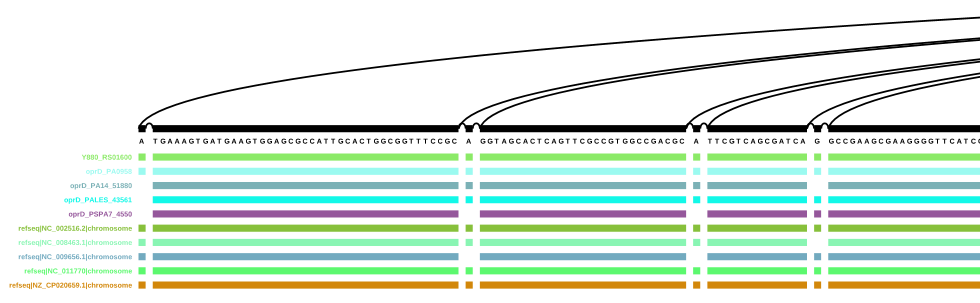
Loading the index into IVG results in an easy answer to my question: Y880_RS01600 is oprD in PAK:
Start of the IVG representation of a sub-graph with all oprD paths
Scrolling through the sub-graph, the path of Y880_RS01600 mostly follows the one of oprD in PAO1, but there are some differences. The same can also be seen in the vg viz representation: vg viz representation of a sub-graph with all oprD paths (SVG)
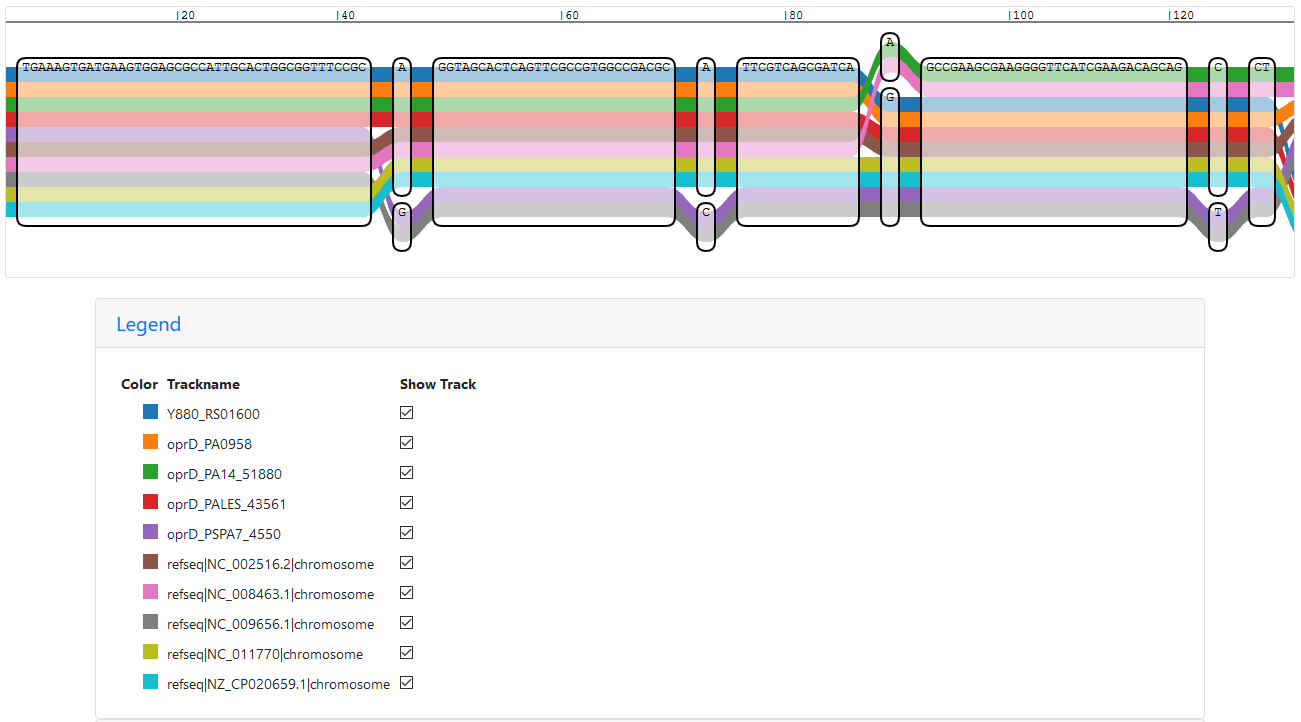
Start of the vg viz representation of a sub-graph with all oprD paths
I’m pretty excited to see that there are no other paths (from all five complete annotations!) found that touch the nodes that are touched by the different oprD genes. If this works with other genes as well, this could be an interesting application to complete genome annotations.
Finding inversions
A question that came up a few times in group discussions about genome graphs was about inversions. In theory, graphs should show even big genomic inversions just fine, but I’m not entirely sure how this works when the basis for the graph is a multiple sequence alignment.
The publication of the PAO1 genome describes a large inversion (more than one-quarter of the genome) compared to a previously mapped isolate, and another publication describes this inversion as being between PA14 and PAO1. It resulted from a homologous recombination event between the rRNAs rrnA and rrnB and should be visible in the graph. The overview generated with odgi viz might already be showing that, but I still find it a little hard to interpret.
A quick check could be to look at either the rRNA clusters where the recombination event took place, or at example genes that are located in the inverted or not inverted parts of the genome. For example, rhl, endocing the ATP-dependent RNA helicase RhlB, is on the positive strand in PAO1 (PA3861), but on the negative strand in PA14 (PA14_14040), while dnaA, encoding the chromosomal replication initiator protein DnaA, as the first gene in the annotation is on the positive strand of both strains.
vg paths -x FivePsaeAnnotAll.xg -X -Q "rhl" > FivePsaeAnnotAll_oprD_rhl.gam
vg view -a FivePsaeAnnotAll_oprD_rhl.gam | jq '{name: .name, nodes: ([.path.mapping[].position.is_reverse | tostring] | join(","))}'
This results in an output of different rhl genes (including rhlR and others) and for each node they touch whether that is reversed or not. The rhl genes (listed for PA14, PAO1, LESB58 and PA7) are all reversed.
Upon closer inspection, this makes sense. The gene might be located in the genomes with different orientations, but it is still read in the same direction, so the path will traverse it in the same direction no matter from which reference it comes.
What about rrnA and rrnB, then? It would be interesting to see the region surrounding those genes. In the PAO1 paper, rrnA is located approximately between bases 722096 and 727255, and rrnB is in the region 4788574 to 4793731. While there is no direct reference to these clusters by name or location in PA14, gene encoding the same features (5S, 16S and 23S rRNA together with tRNA for alanine and isoleucine) can be found in similar regions: 733095 to 738251 and 4952020 to 4957169.
It’s a pity that it’s not possible to simply find these genomic locations in the graph, and I think it’s also not possible to select a gene/feature and to specifically extract its surroundings, as I believe this only works with node IDs. Therefore, I will have to either decide which nodes to extract, or which annotated features.
Open questions
- Is there another way to visualise a whole genome graph?
- How can I annotate the graph? Is a specific formatting of GFF files required?
- The files just have to strictly follow the specifications, I believe.
- How does
vg vizwork compared tovg view (-d)? Are the nodes sorted differently, and if so, why? - How does
vg find -Nwork? Why are more nodes included than were on the list? - What exactly happens when multiple paths have the same or no name (i.e. annotation of genes with the same name, or no name)?
Back to main page.